Tutorial

• Introduction

• Running METALoci on example data

  • Downloading the data

  • Generating a metaloci region file

  • Binning the signal files

  • Layouting the Hi-C matrix

    • Finding the best parameters

    • Running ‘metaloci layout’

  • Computing the spatial autocorrelation of the signal

  • Plotting the results

    • Interpreting the results

Introduction

METALoci is a tool to systematically identify spatial autocorrelation of signals in the 3D genome. Hence, to use METALoci we will need Hi-C data (.cool, .mcool, and .hic formats are supported) and a signal track (e.g. ChIP-seq, ATAC-seq, etc.) in .bed format. We will need some additional files to run the pipeline, but we will guide you on how to find/generate them in the following sections.

METALoci is a command-line tool, so you will need to have some basic knowledge of how to use the terminal. Advanced users may also want to create their owns scripts by using the METALoci Python API, but we will not cover that in this tutorial.

This package has several submodules that we can invoke from the command line. These submodules are:

• metaloci: The main module of METALoci. You can see a brief explanation of the available commands by running it.

• metaloci prep: Processing of the .bed signal files for them to be used in METALoci.

• metaloci layout: Generation of the Kamada-Kawai layouts, given a Hi-C matrix and a list of regions to process.

• metaloci lm: Calculation of the spatial autocorrelation of the signal given the previously calculated layouts.

• metaloci figure: Plotting of the results of the pipeline.

Additionally, we have a few QoL scripts that can be used to generate necessary files, find the best parameters for the run, and some downstream analysis. These are:

• metaloci sniffer: Given a .gtf file for a specific genome, generate a metaloci region file with the coordinates of the genes, genome-wide.

• metaloci bts: Given a Hi-C matrix and a resolution, determine the best values of cut-off and persistence length for the run.

• metaloci gene_selector: Given an already processed working directory, selects regions whose point of interest is significant according to a given threshold.

In the following sections, we will guide you on how to use these submodules and scripts to run METALoci with some example data.

Note

If you have not already done so, you may install METALoci by following the Installation instructions.

Running METALoci on example data

Downloading the data

To run METALoci, we will need some example data. You can download it with:

git clone https://github.com/3DGenomes/METALoci && mv METALoci/metaloci/tests/data . && mv METALoci/docs/tutorial.ipynb . && rm -rf METALoci

This will download the example data to a folder named data in your current working directory. The data consists of a Hi-C matrix, a few ChIP-seq signals, and a .gtf file to generate the region file.

Generating a metaloci region file

The first step is to generate the metaloci region file. This file contains the coordinates of the regions we want to process. The structure of the file is as follows:

coords  symbol    id
chr19:41370000-45380000_200 Crtac1  ENSMUST00000238290.2
...

Where:

• coords: The coordinates of the region. poi stands for point of interest, and it is the bin of the Hi-C matrix that will be highlighted in the results. It can be a dummy number if you do not have a specific bin in mind.

• symbol: Name of the gene contained in the region.

• id: ENSEMBLE ID of the gene.

You can manually build this file if you do not have many regions to process. However, if you have a lot of regions, you can use the metaloci sniffer script to generate it. The script requires a .gtf file for the genome you are working with. You can download the .gtf file for the mouse genome from GENCODE. For example, for the mouse genome (mm39), you can download the file from GENCODE and then click on Comprehensive gene annotation -> GTF.

You will also need a file with the chromosome sizes. You can download this file from the UCSC Genome Browser. For the mouse genome (mm39), you can download the file from UCSC and save mm39.chrom.sizes as a txt file. This file is already in the example data, so you do not need to download it again.

For the sake of speed, we will use the .gtf file provided in the example data. This is a subset .gtf file that only contains the regions of chromosome 19. You can generate the region file with:

metaloci sniffer -w example_working_directory -s data/mm39_chrom_sizes.txt -g data/gencode.vM39.annotation_chr19.gtf.gz -r 10000 -wi 4000000

Note

The ‘’.gtf’’ file name could change depending on the version you download from GENCODE.’

When prompted, select ‘protein coding’, with 6 + ENTER. This should create a new working directory and create a metaloci region file inside it.

The -r flag is the resolution of the Hi-C matrix. It is recommended to use the highest resolution your Hi-C matrix can provide. The -wi flag is the size of the region that will be processed centered around the TSS, our point of interest. These two parameters will determine the number of bins the Kamada-Kawai layout will have (in this case, 4000000 / 10000 = 400 bins)

Note

The recommended amount of bins is around 400. In this case, 4Mb 4000000 / 10000 = 400 bins.

A number of bins higher than 900 is not recommended.

You can read more about this script in the Command Line Interface section.

Binning the signal files

In order to be able to use the signal files in METALoci, we need to bin them. This is done with the metaloci prep script. This script will take the signal files and bin them according to the Hi-C matrix resolution. It will then take care of assigning the proper ‘amount of signal’ to each bin if the signal is already binned to a higher resolution. If multiple files are provided, the script will merge them into a single file. If the bed files do not have a header, the name of the signal will be the name of the file. You need to provide the Hi-C matrix you will be using in further steps in order to check for consistency in the nomenclature of chromosomes. To bin the signal files, run:

metaloci prep -w example_working_directory -c data/hic/ICE_DM_5kb_eef0283c05_chr19.mcool -d data/signal/mm39_organoid_ATAC_4000_chr19.bed -r 10000 -s data/mm39_chrom_sizes.txt

This will create a new folder called signal inside the working directory.

Note

The -r flag is the resolution at which the signal files will be binned. This resolution must be the same as the resolution used in the region file and must be available in the provided Hi-C file.

Note

If you happen to have a very big signal file (i.e. very high resolution ChIP-seq data for a lot of different marks), this script may take a long time to run and use a large amount of memory. The biggest signal file that has been tested consisted of a 67 G .bed file with 11512 different signals. It required ~300 G of memory in an HPC environment and took ~30 hours to run. With a smaller signal file, the script should run in a few minutes (or even a few seconds).

You can read more about this script in the Command Line Interface section.

Layouting the Hi-C matrix

Finding the best parameters

Note

As of METALoci v1.2.0, a new way of estimating the best parameters for the layout has been implemented. ‘metaloci bts’ will still be available, but using the flag ‘-i’ in ‘metaloci layout’ is the prefered way of estimating the best parameters.

We have already chosen the resolution of the Hi-C matrix and the size of the region. However, we still need to find the best values for the cut-off and the persistence length. The cut-off is the minimum value of the Hi-C matrix that will be considered in the layout. The persistence length is a value of the ‘stiffness’ of the layout, that corresponds to the minimum distance between two consecutive particles in the layout. The higher the value, the more ‘stiff’ the layout will be. To find the best values for these parameters, we will use the metaloci bts script:

metaloci bts -w example_working_directory -c data/hic/ICE_DM_5kb_eef0283c05_chr19.mcool -r 10000 -g example_working_directory/example_working_directory_protein_coding_2000000_10000_gene_coords.txt

This script may take a few hours, depending on the computing power of your PC. Once you have determined the best values for your Hi-C you will not need to run this script ever again. You can skip running this script for the sake of speed. The output parameters for this run would be cut-off = 0.2 and persistence length = 7.044.

You can read more about this script in the Command Line Interface section.

Running ‘metaloci layout’

Now that we have all the necessary files, we can run the metaloci layout script. This script will generate the Kamada-Kawai layout for the Hi-C matrix. The script would use the metaloci region file that has been computed by metaloci sniffer, that contains all the regions in chromosome 19. for the sake of speed, we will make a subset to only process the first 16 regions. To subset the file, run:

{ head -n 1 example_working_directory/example_working_directory_protein_coding_4000000_10000_gene_coords.txt; tail -n +2 example_working_directory/example_working_directory_protein_coding_4000000_10000_gene_coords.txt | shuf -n 16; } > example_working_directory/example_working_directory_protein_coding_2000000_10000_gene_subset_coords.txt && rm example_working_directory/example_working_directory_protein_coding_2000000_10000_gene_coords.txt

And then run the layout script, which will automatically recognise the new region file:

metaloci layout -w example_working_directory -c data/hic/ICE_DM_5kb_eef0283c05_chr19.mcool -r 10000 -o 0.2 -l 7.044

Alternatively, you can use the flag ‘-i’ to automatically estimate the best parameters for each region. You can omit the -o, the -l or just one of them, and it will be automatically estimated:

metaloci layout -w example_working_directory -c data/hic/ICE_DM_5kb_eef0283c05_chr19.mcool -r 10000 -i

Note that using ‘-i’ several times in one region might slightly change the results, as the way the cut-off is estimated is not deterministic.

If you wish to use another metaloci region file, you can specify it with the -g flag. You can also specify a single region rather than using a whole region file (e.g. chr19:2310000-6320000_200). The -m flag will set the use of multiprocessing, to make things quicker. If you want more information printed on the screen, omit this flag (things will get slower).

This script will generate a .mlo file for each region. This file is a pickle of an object that contains information about the region, the matrix, the processed Kamada-Kawai layout, etc. You can read more about this file in the METALoci Python API, in the metaloci.mlo module.

Note

You can use the flag -p to plot the Kamada-Kawai and check everything looks alright. You will find these plots in the plots folder inside the chromosome folder.

You can read more about this script in the Command Line Interface section.

Computing the spatial autocorrelation of the signal

Once we have our signal binned and the Kamada-Kawai layout generated, we can compute the spatial autocorrelation of the signal using Local Moran’s Index. To do this, we will use the metaloci lm script:

metaloci lm -w example_working_directory -s mm39_organoid_ATAC_4000_chr19 -b

With the argument -s we can specify which signal we want to process. You can also specify a file with the names of multiple signals, one per line. If you do not know the exact name of the signal, you can find it in the signal folder. The -b flag will output metaloci bed files, with the location of the bins with significant autocorrelation of the quadrants we specify.

Note

The script will process all the regions in the region file, but you can specify another region file with the flag -g. The -m flag will set the use of multiprocessing, to make things quicker. If you want more information printed on the screen, omit this flag (things will get slower). The -q argument, allows you to specify the quadrants that you will consider important in your run (default is quadrants 1 and 3). The flag -i will ‘unpickle’ all the information about the run in a .txt file.

You can read more about this script in the Command Line Interface section.

Plotting the results

METALoci includes a script to plot the results of the pipeline. metaloci figure will compute the following plots:

• Hi-C matrix.

• Signal plot: Distribution of the signal values along the region.

• Kamada-Kawai plot.

• Local Moran’s I scatter plot. X axis corresponds to the signal, Y axis corresponds to the signal lag.

• Gaudí signal plot: Voronoi-based representation of the distribution of the signal in the layout.

• Gaudí type plot: Result of the autocorrelation analysis, with the significant bins highlighted.

To plot the results, run:

metaloci figure -w example_working_directory -s mm39_organoid_ATAC_4000_chr19 -z

You can check the plots in the plots folder inside the chromosome folder. A ‘composite’ image with all the plots will also be generated.

Note

There are few additional arguments regarding the highlight of the plot, significance threshold, quadrant to be considered important, etc. You can check them out in the Command Line Interface section.

Interpreting the results

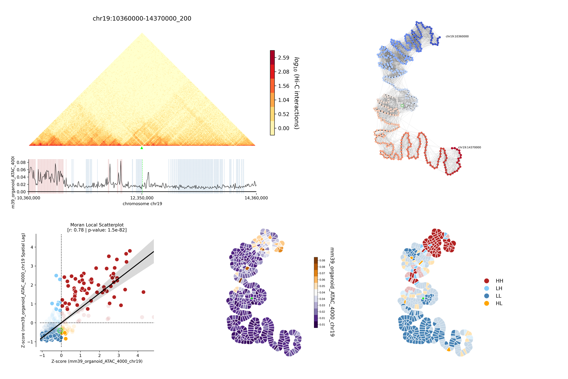
Example output for region chr19:41370000-45380000_200 in mm39 myeloid cells with ATAC-seq.

The composite figure shows the results of the pipeline for a single region. The following plots have been generated:

• The first plot is the Hi-C matrix, with the region of interest highlighted.

• The second plot is the signal plot, showing the distribution of the signal along the region. The signal plot has been highlighted according to significant metalocis –regions with a spatial correlation of the signal– found in the run.

• The scatter plot represents a linear correlation between the signal of a bin (x axis) and the signal of its neighbours (y axis), where only the significant bins have a solid colour. The plot is divided into four different quadrants, according to the spatial autocorrelation of the signal:

  • Quadrant 1: High signal, high signal lag. -> HH

  • Quadrant 2: Low signal, high signal lag. -> LH

  • Quadrant 3: Low signal, low signal lag. -> LL

  • Quadrant 4: High signal, low signal lag. -> HL

• The Kamada-Kawai layout is just a representation, in a 2D layout, of the information of the Hi-C for that particular region, without taking into account the signal.

• The Gaudí signal plot is a representation of the spatial distribution of the signal in that layout.

• The Gaudí type plot is the result of the autocorrelation analysis, with the bins in the colour that corresponds to its quadrant in the scatter plot. The significant bins have, again, a solid colour, while the non-significant bins have some transparency.

Note

You can systematically detect metalocis for the regions you process using the -b flag in metaloci lm. This will create .bed files with the locations and type of the metalocis found in the run. You can use these files to do some downstream analysis. You may also want to use the metaloci gene_selector script to select regions whose point of interest is significant according to a given threshold. You can also extract more information about the run using the -i flag in metaloci lm to generate a .txt file per region.